Machine Learning using FluxML
This example is taken from Randy Davila. The original is available on the TalkJulia website: https://www.talkjulia.com/ (with only minor tweaks).
This is a really good resource!
using Flux
Preparing the Training Data
# Target Function
target_function(x) = @. 4x + 2

# Create Artificial Data
# Note! These are row feature vectors
x_train, x_test = hcat(0:5...), hcat(6:10...)

# Apply the target function to the test and train row vectors
y_train, y_test = target_function(x_train), target_function(x_test)
([2 6 … 18 22], [26 30 … 38 42])
scatter(x_train, y_train, color = "magenta", legend = false)
x_train
1×6 Matrix{Int64}:
 0  1  2  3  4  5
y_train
1×6 Matrix{Int64}:
 2  6  10  14  18  22
The Single Artificial Neuron Model
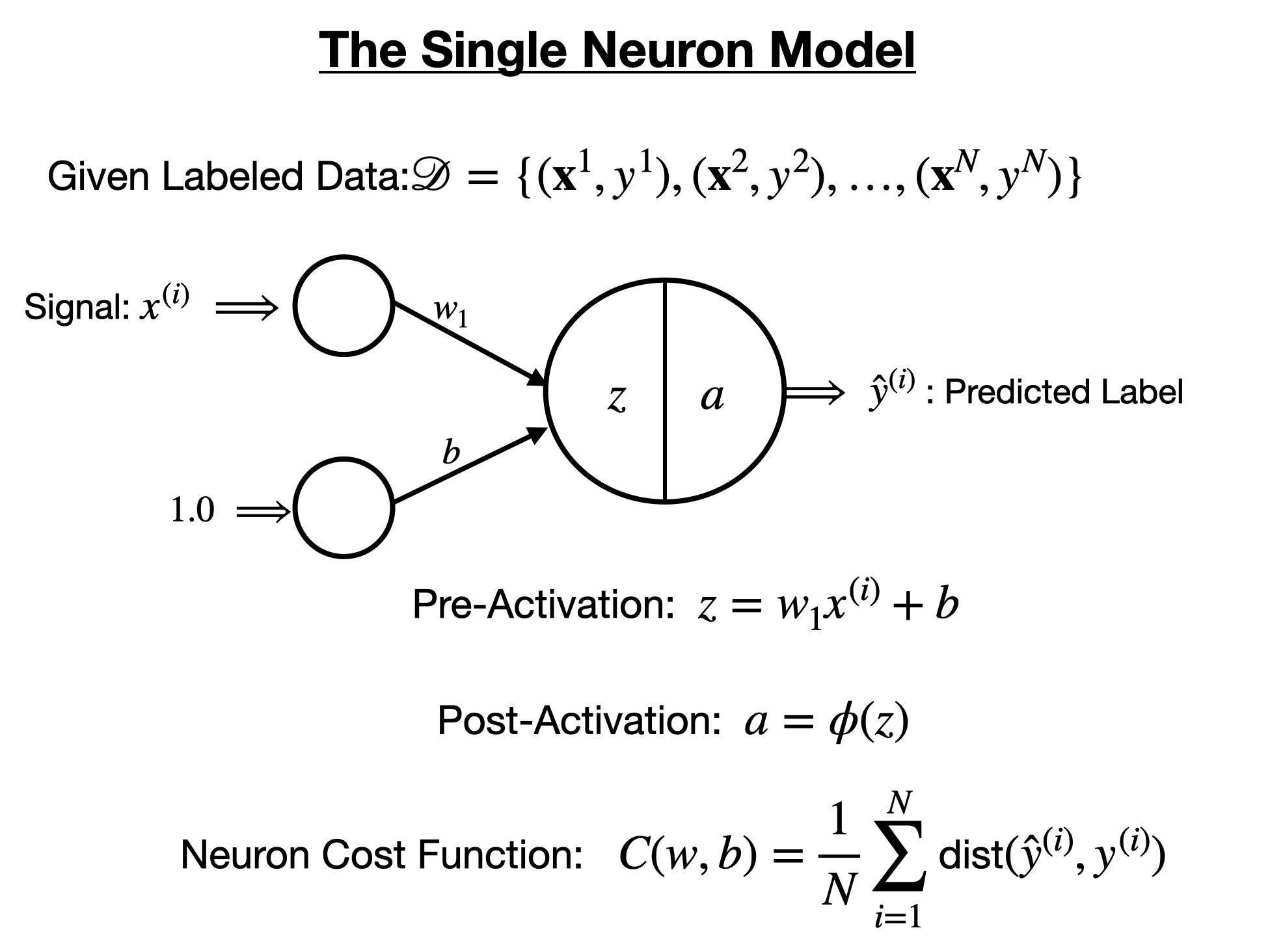
A single artificial neuron is a computational unit, or function, that takes as input a feature vector, and outputs a real value in the case of regression, or a label in the case of classification. The single neuron model consist of several fields depicted in the figure below.

We can create a single artificial neuron with one weight and one bias using Flux.jl.
# Define a simple model with one input node
model = Flux.Dense(1, 1)

println("model weight variable = $(model.weight)")
println("model bias variable = $(model.bias)")
model weight variable = Float32[-0.8471055;;]
model bias variable = Float32[0.0]
Single artifical neurons are functions, and Flux.jl treats them as such:
# Models are predictive functions
model(x_train)
1×6 Matrix{Float32}:
 0.0  -0.224625  -0.44925  -0.673875  -0.8985  -1.12313
For linear regression, it is standard to set the loss function of our single neuron to be the mean squared error function: $ MSE(X, y) = \frac{1}{2N}\sum_{i=1}^N(\hat{y}_i - y_i)^2 $
We can define this loss function with the following code:
# Define Mean Squared Error Loss Function
loss(x, y) = Flux.Losses.mse(model(x), y)

println("Current Loss = $(loss(x_train, y_train))")
Current Loss = 209.84795
In order to train, or update, the single neurons weights and bias to minimize the loss function we need to define an optimizer, such as gradient descent, or ADAM. We will also need to format are training data as an Array of tuples $(x, y)$, and gather the weights and bias of the single neuron.
# Define Gradient Descent Optimizer
opt = Flux.Descent(0.01)

# Format your Data
data = [(x_train, y_train)]

# Collect weights and bias for your Models
parameters = Flux.params(model)
Params([Float32[-0.224625;;], Float32[0.0]])
Now that we have a loss function, parameters to be trained, training data, and an optimizer, we can next train our paramaters to decrease the loss function of the model:
println("Old Loss = $(loss(x_train, y_train))")

# Train the model over one epoch
Flux.train!(loss, parameters, data, opt)

println("New Loss = $(loss(x_train, y_train))")
Old Loss = 209.84795
New Loss = 135.23073
Suprisingly, Flux.Decent() is full gradient descent. In practice this can be very slow, so we adapt this optimizer to implement stochastic gradient descent as follows:
println("Old Loss = $(loss(x_train, y_train))")
(m, n) = size(x_train)
epochs = 1_000
losses = Float64[]
for _ in 1:epochs
    for i in 1:n
        Flux.train!(loss, parameters, [(x_train[:, i], y_train[:, i])], opt)
        new_loss = loss(x_train, y_train)
        print("New Loss = $(new_loss) \r")
        push!(losses, new_loss)
    end
end
Old Loss = 135.23073
New Loss = 2.1221542e-12
plot(losses, yaxis=:log)
scatter(x_test, y_test, color = "magenta")
domain = LinRange(6, 10, 100)

plot!(domain, domain .* model.weight .+ model.bias, legend = false)